Sorting and Aggregates
Sorting
What is sorting?
Sorting is just arranging elements in a specific order. But why is this important for database management systems (DBMS)?
Why does sorting matter in DBMS?
DBMS needs sorting for two main reasons:
- SQL uses the
ORDER BYclause to return data in a specific order. - Sorting helps make query processing more efficient. When records are sorted, operations like joins and
ORDER BYcan be done faster.
Types of sorting:
There are two ways data can be sorted: physically and virtually.
Physical sorting means the data is actually stored on the disk in sorted order.
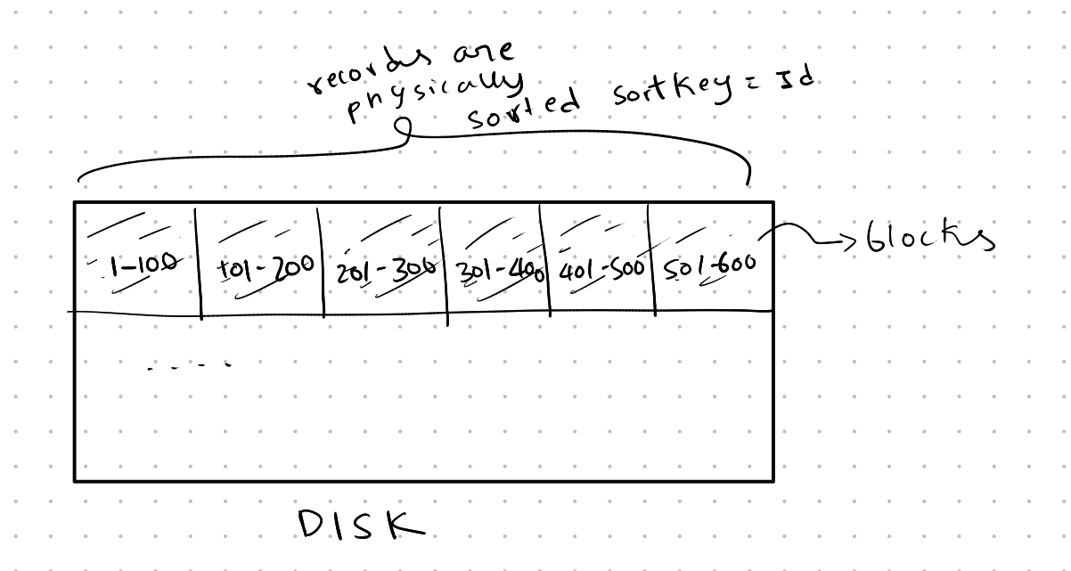
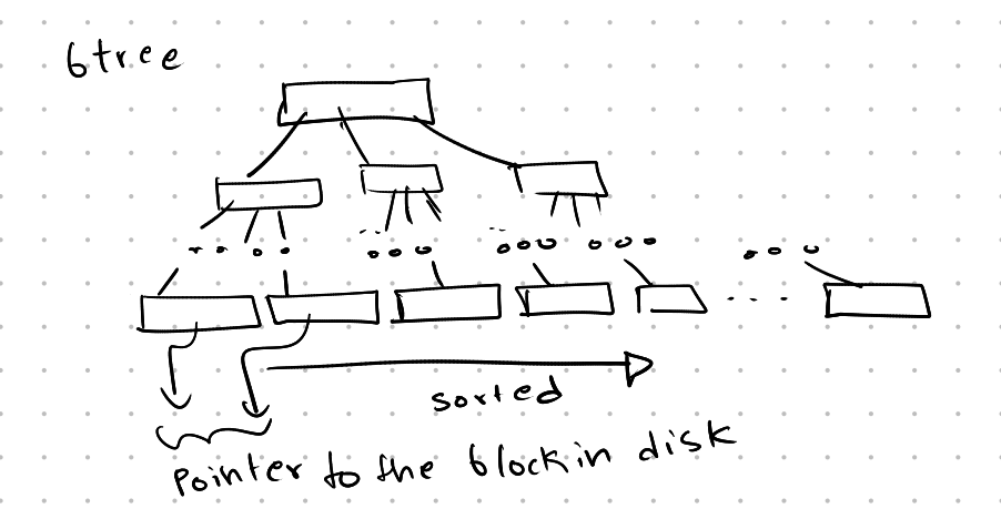
Virtual sorting refers to the logical arrangement, like in a sorted B-Tree. Here, the records are arranged in order for quick access, but the physical storage on disk might not be sorted the same way.
Why does physical sorting matter?
Imagine you sorted records based on a certain key and now need to access them one by one. If the physical sort order is different from the logical order, it will cause random disk I/O operations, which are slow. Disks perform much better with sequential access rather than random access.
In a clustered B-Tree, the sort key used in the B-Tree is the same as the physical sort order on disk, leading to faster access.
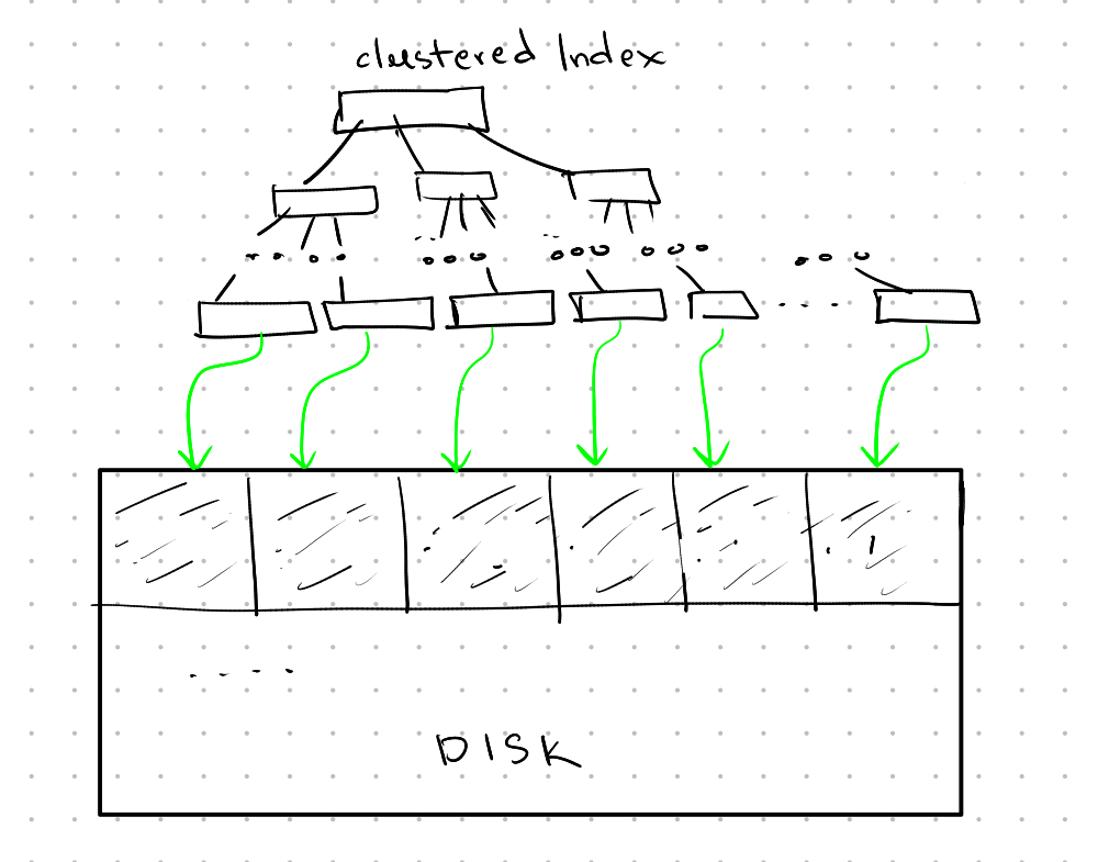
In an unclustered B-Tree, the sort key of the B-Tree differs from the physical order on disk, causing slower random access.
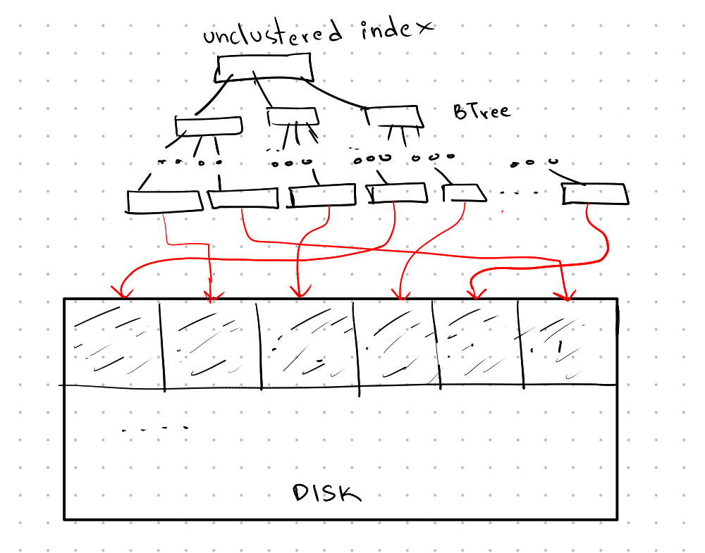
We know that the data in a database can be much larger than the available memory. Sorting data that doesn’t fit in memory is called external sort.
Some common sorting algorithms include:
- Top N Heap Sort: This algorithm is used when we want to get the top N rows from the results. It works by creating a heap of size N and going through the rows to update the heap.
- Time complexity: O(n log n)
- Space complexity: O(1)
- Here is a great video if you want to learn more about heap sort: https://youtu.be/HqPJF2L5h9U
- Quick Sort: Quick sort organizes elements by dividing them around a chosen pivot.
- Time complexity: O(n log n)
- Space complexity: O(n)(The time and space complexity of quick sort depend on how the pivot is chosen.)
- Insertion Sort: Insertion sort is a simple algorithm where elements are added one by one into a sorted array. It’s similar to sorting playing cards.
- Time complexity: O(n²)
- Space complexity: O(1)
- Merge Sort: In merge sort, the array is divided into two halves, and each half is divided again until we have single elements. Then, these parts are merged back together to create a sorted array.
- Time complexity: O(n log n)
- Space complexity: O(n)
The choice of sorting algorithm also depends on the initial arrangement of the elements. For example, if the elements are mostly in reverse order, simpler sorting algorithms like Insertion Sort and Bubble Sort perform much better. However, this is not always the case.
How to Sort Large Data Sets
When the data to be sorted is too large to fit in memory, we use a technique called external merge sort.
External Merge Sort
External merge sort has two main phases:
Creation of Runs:
In this phase, “runs” refer to chunks of sorted pages. A one-page run means the size of the run is one page, and the elements in that run are sorted. A two-page run means the size is two pages, and the elements in those two pages are also sorted, and so on.

Merge of Runs:
In this phase, we merge two or more runs together to create a new run where all the elements are sorted. The size of the new run is equal to the total size of the previous runs that were merged.
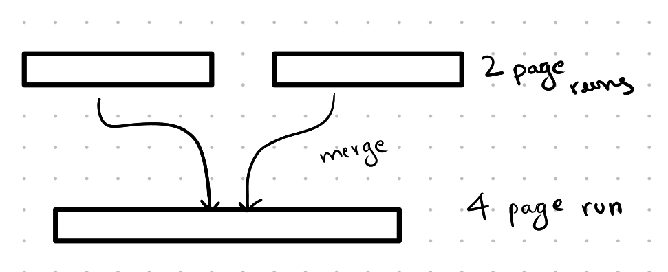
Example of External Merge Sort
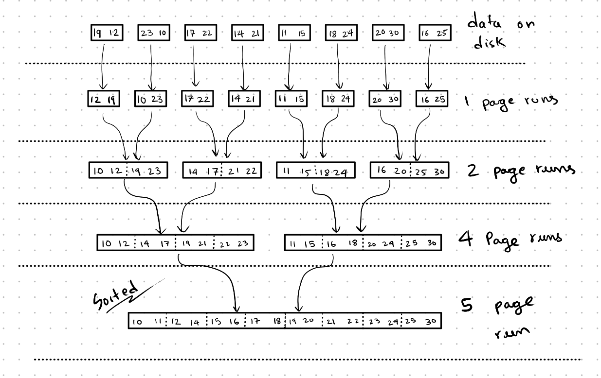
Let’s say we have 8 pages of data to sort, but our memory can only hold 3 pages at a time.
Creation of Runs:
First, we load all the pages into memory and sort them using an in-memory sorting algorithm based on our needs. After sorting, we store these pages back on the disk, which we will call one-page runs.
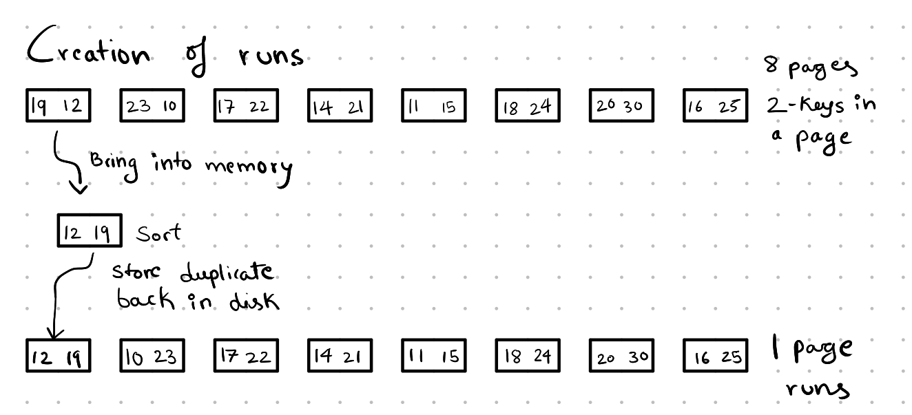
Merging Runs:
Next, in the merge phase, we load 2 pages, one from each run (here each run has only one page). With only 3 pages of memory available, we use one page to store the output. We then merge the two pages into the third page. When the output page is full, we write it back to disk. After finishing with the page from the run, we load the next page from the run, similar to the merge step in the merge sort algorithm.
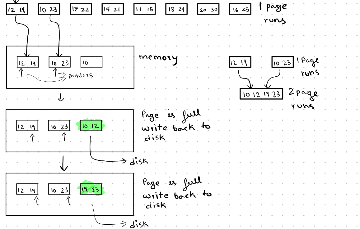
Continuing the Process:
Now that we have two-page runs, we repeat the process by loading one page from each of the two-page runs into memory and merging them into a single page. We then write this back to the disk. When we finish with a page, we load the next page from the run and continue this process.
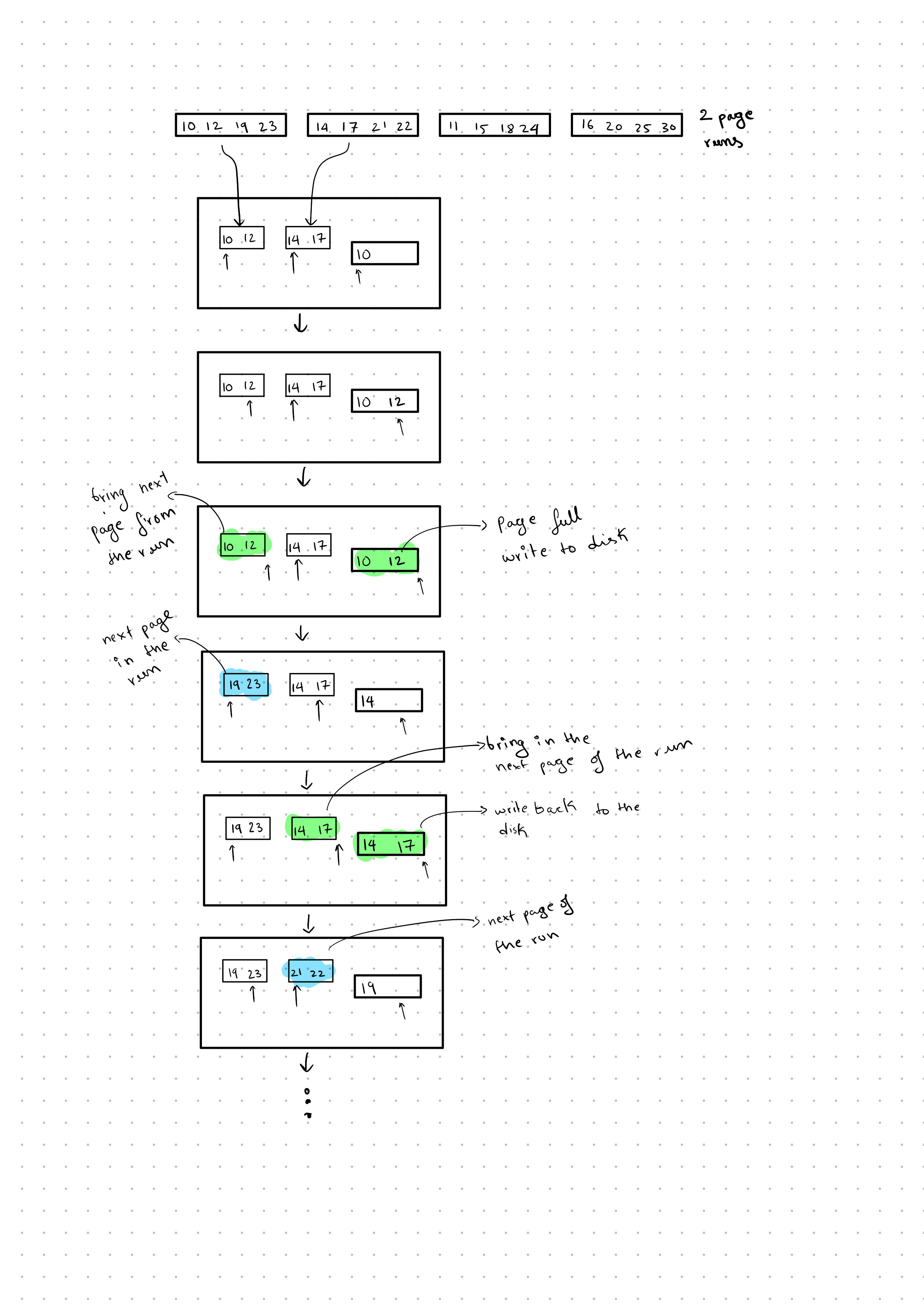
This process continues until all the data is sorted.
Cost Analysis of External Merge Sort
The external merge sort algorithm has two main components: the number of passes and the number of I/O operations. For each pass, we perform 2*N I/O operations: N read operations to load the pages into memory from disk and N write operations to save the sorted pages back to disk. While we cannot reduce the number of I/O operations, we can optimize the number of passes.
In the algorithm we discussed earlier, during each pass, we merge 2-page runs to form 4-page runs, and so on. This means the total number of runs is halved with each pass. It’s important to note that a 4-page run means there are 4 pages in that run, not 4 separate runs. This was a bit confusing for me initially.
The total number of passes can be expressed as $\log_2(N) + 1$ , where the “+1” accounts for the initial pass where we sort the individual pages. In this case, we have only 3 pages in the buffer. However, if we have B pages in the buffer, we can merge B-1 runs at a time (k-way merge). During the initial pass, we can load B pages into memory and sort them directly, producing B-page runs. Therefore, we start merging with $\lceil \frac{N}{B} \rceil$ , leading to the new equation:
$$ log_{B-1}(\lceil \frac{N}{B} \rceil) + 1 $$
We know that disks perform better with sequential access rather than random access. Previously, we only brought one page from a run into memory. This caused the disk head to move around a lot to retrieve a page from each run. To minimize this, we can load multiple pages from the same run at once, reducing random accesses. However, this comes with a trade-off: it limits the number of runs that can be merged at a time. For example, if we have 9 pages and bring in a single page from each run, we can merge 8 runs at once. But if we load 2 pages from a single run, we can only merge 4 runs at a time.
If we load chunks of pages from a run, say C pages, the equation becomes:
$$ log_{\frac{B}{C}-1}(\lceil \frac{N}{B} \rceil) + 1 $$
Having a larger buffer significantly speeds up the sorting process. Let’s calculate the number of passes for ( N_1 ) (number of pages) = 1,000,000 and ( B_1 ) (buffer size) = 3, and for ( N_2 ) = 1,000,000 and ( B_2 ) = 50.
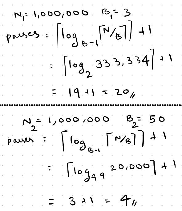
We can clearly see that increasing the buffer from 3 to 50 reduces the number of passes from 20 to just 4.
Optimizations
Double Buffer Optimization
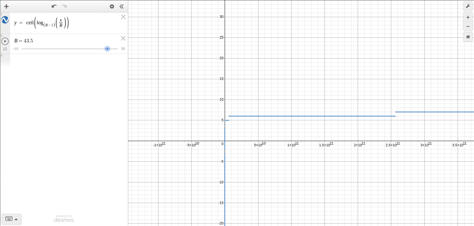
From the graph below, we can see that the output remains consistent over a large range of pages. Changing the buffer size only slightly affects the number of passes. While merging, the disk can remain idle. However, we can allocate some buffer pages for pre-fetching from the disk. This way, while merging is happening, the disk can load the next batch of pages into memory, speeding up the process.
Comparison Optimizations
Some comparisons can also be optimized using specialized code. For example, if the data type is a string, instead of comparing the entire length of two strings, we can first compare just the first n characters. This can reduce the number of operations required.
Aggregates
In aggregates, the result is produced by performing calculations over several elements, such as count, max, min, etc.
If an ORDER BY clause is used in the query, we need to sort the data. To do this, we can use the external merge sort method to order the elements.
If there is no ORDER BY clause, we can use hashing, which is generally faster than sorting.
Like sorting, hashing has two phases:
Partitioning:
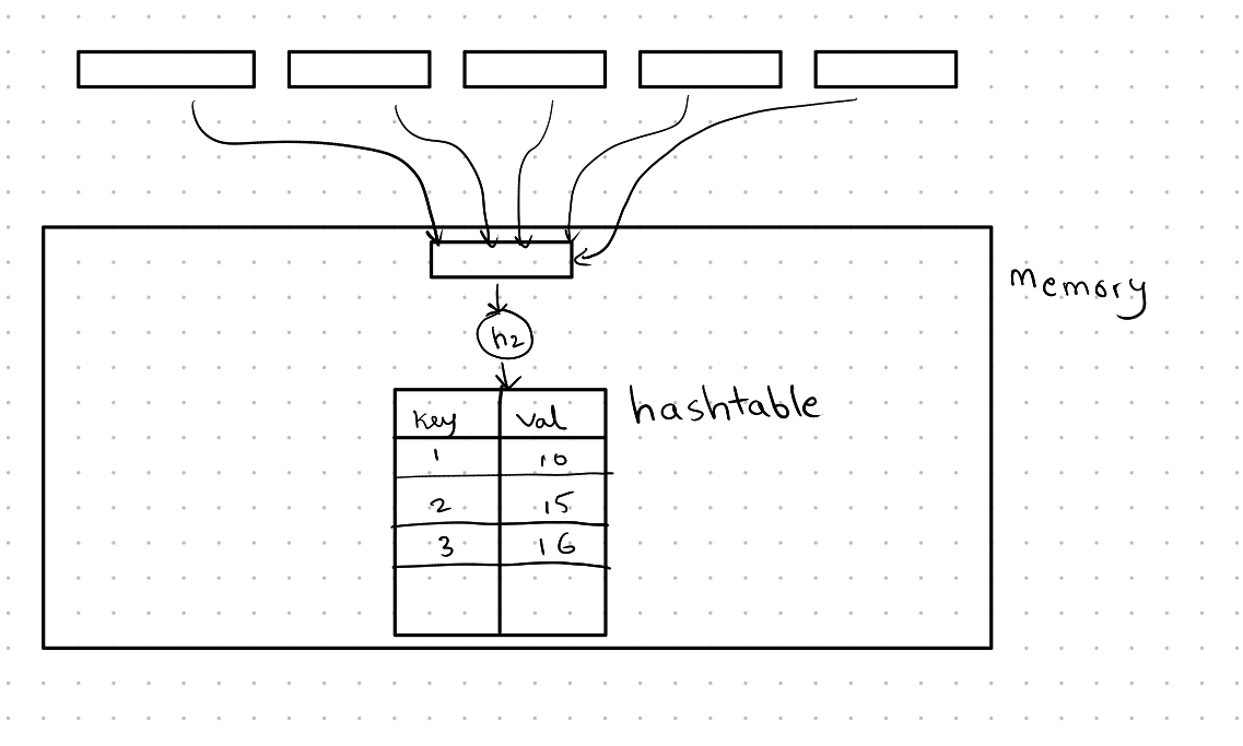
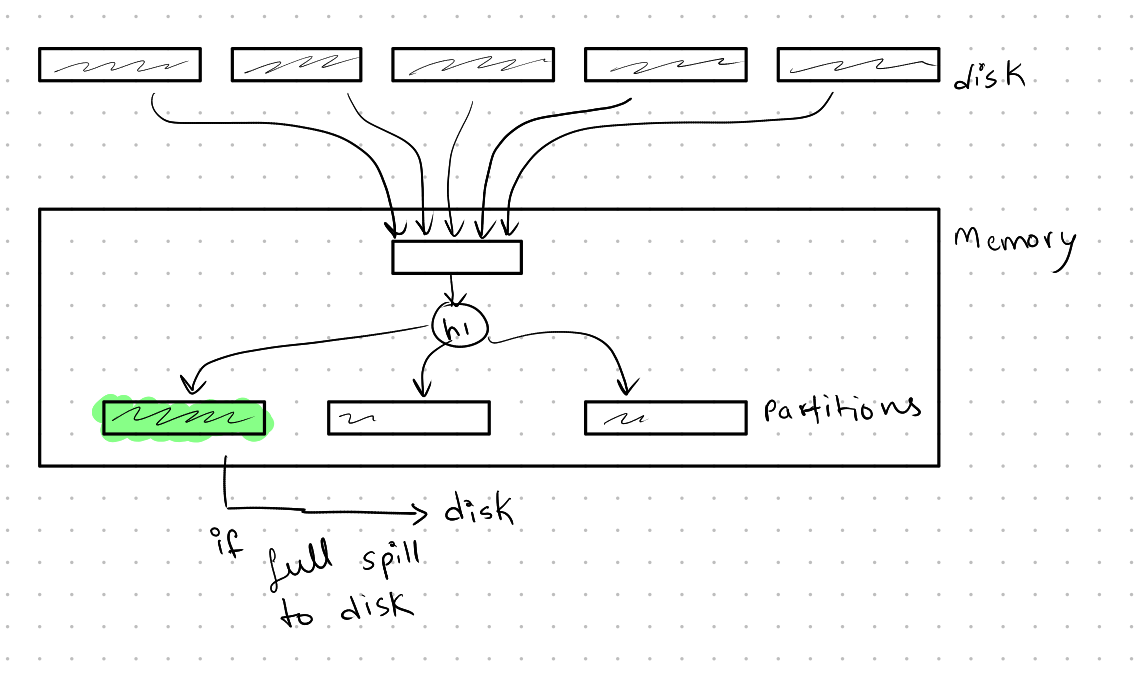
In this phase, we partition the data into several chunks. The number of chunks is equal to B-1, where B is the number of buffer pages available. When we bring a page from the disk, we hash it to one of the pages using a hash function, say ( h_1 ). If the page overflows, we spill it to disk, creating several partitions.
Reparation:
In this phase, we bring in pages from each partition and hash them using another hash function, say ( h_2 ). Depending on the required aggregate operation, we might store a running sum of the necessary values. For example, if we want to calculate the average grade grouped by the course, we would store the running sum of the number of students in the course and the total sum of the students’ grades. This information can then be used to calculate the final result.
The example below shows how we might store the course ID (key) and the total number of students in that course.
