Map-Reduce

Before getting into MapReduce, let’s first understand what distributed systems are — and why they’re widely used.

Imagine You have some work that can be done by a computer. What do you do? Easy — you just assign the work to your computer. Now the work gets harder, and it’s taking longer to complete. What do you do? Simple — buy a better CPU, GPU, more RAM. Upgrade your computer. That’s awesome. But then the work gets even harder. What now? You upgrade again — even better CPU, GPU, and RAM. Now you’re running the latest, top-notch machine. You’ve maxed out how strong your computer can be. But the work keeps growing. It takes more time again. And now, you can’t make your computer any stronger. Looks like we’ve hit a wall, right? Actually… no. What if we make two computers do the work? Hmmmm. And if the work grows again? Just add two more computers. Then four. Then ten. This is called horizontal scaling — adding more machines instead of upgrading just one. And when multiple computers work together on a problem, we call that a distributed system.

So what is MapReduce, and how does it fit into distributed systems?

Think of MapReduce as a ninja technique that helps us split up work across multiple computers and stitch the results back together — all while making the process faster and more efficient.

Let’s break it down with an example.

The Problem: Sum of Numbers Across Multiple Computers

Imagine you have 10 computers, and each stores 100 numbers.

Computer 1: numbers 1–100
Computer 2: numbers 101–200
… and so on.

Now, you want to compute the sum of all 1,000 numbers.

Naive Approach:

You let one computer do the work. It asks the other 9 for their numbers over the network.

If it takes:

1 second to add two numbers
0.1 second to fetch a number from another computer
0 seconds if the number is already local

Here’s the catch:

Only 100 numbers are local. The remaining 900 need to be fetched.

First 99 additions (local): 99 seconds
Next 900 additions (remote): 900 × (1 + 0.1) = 990 seconds

Total time: 99 + 990 = 1,089 seconds

That’s sloooow.

MapReduce-Style Approach:

Now, What if each computer adds up its own 100 numbers in parallel?

Computer 1: sum = 5050
Computer 2: sum = 15050
Computer 3: sum = 25050
… and so on.

Each computer performs 99 additions locally (no network delay).

Time taken per computer: 99 seconds

Once done, they send their 10 partial results to Computer 1.

Sending 9 results: 9 × 0.1 = 0.9 seconds
Final 9 additions: 9 seconds

Total time: 99 + 0.9 + 9 = ~108.9 seconds

That’s 10 times faster!

As you can see, the MapReduce style has two key phases:

The phase where each computer adds up the numbers that are local to it — this is called the Map Phase.
The phase where all computers send their local results to one computer for the final showdown — this is the Reduce Phase.

Now let’s get into the technical details of how map reduce actually work…!!! master, preprocess and create tasks map tasks, reduce tasks, workers ask for tasks send results to master, fault tolerance,

Now, let’s dive into some technical details of how MapReduce is actually implemented.

How does MapReduce work?

Imagine you own a massive digital library with 100 terabytes of .txt files distributed across 10 computers.

Your task is to count how many times a particular word appears across all the books.

To do this efficiently, you can use MapReduce. But before we get started, we need to define two functions: the Map function and the Reduce function.

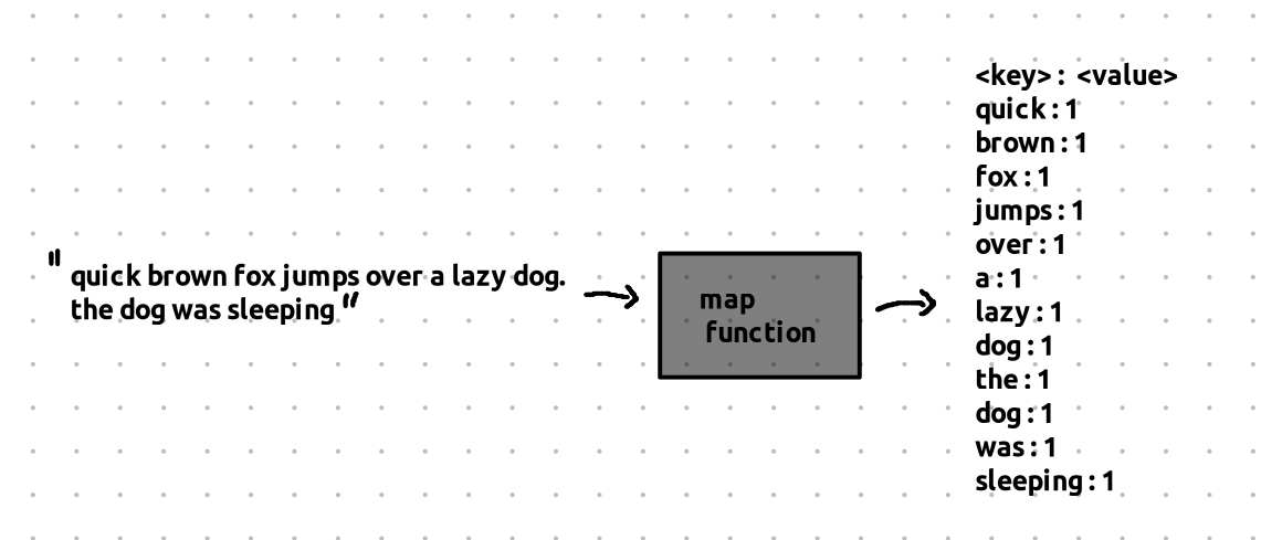
What is a Map Function?

The Map function takes a portion of the text and maps it into key-value pairs. These key-value pairs are also known as intermediate key-value pair

Now, what exactly should the Map function do?

It will break down a chunk of text (from one of the files) and produce a key-value pair for each word in that text.
The key will be the word itself.
The value will always be 1 (because we’re just counting the occurrences of each word).

So, if the word “dog” appears 2 times in a particular block of text, the Map function will output:

Key: “dog”, Value: 1 (for each occurrence).

What is a Reduce Function?

It takes all key-value pairs that share the same key and combines them into a single result.

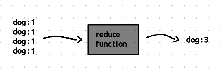
For instance, if we have many key-value pairs for the word “dog”, like:
- “dog” → 1
- “dog” → 1
- “dog” → 1
- “dog” → 1

The Reduce function will combine these values and output a single pair:

Key: “dog”, Value: 4 (the total count of the word “dog” across all the chunks).

How Does MapReduce Work in Practice?

Now that we have our Map and Reduce functions, let’s look at how MapReduce actually runs in a distributed system to give us the results we want.

For simplicity, let’s assume the master and reducers are separate computers. But in reality, the workers themselves perform the reduce tasks, and the master is only responsible for task assignment and monitoring.

The Master and Worker Computers

In a MapReduce system, we have two types of computers:

Master Computer: The job of the master is to assign tasks to the worker computers.
Worker Computers: These are the machines that actually process the data and perform the work, running the Map and Reduce functions.

But how does the master know which task to assign to which worker? Here’s where things get clever.

Task Assignment and File Distribution

Each worker computer needs to access the data stored on the network, but if the required file is not on the computer, it would need to fetch it from another machine. Network transfer is slow, so we want to minimize this delay.

The Master Computer is smart. It knows exactly where the data is stored and assigns tasks so that, as much as possible, the worker computers can access the required data locally, without the need for network transfers.

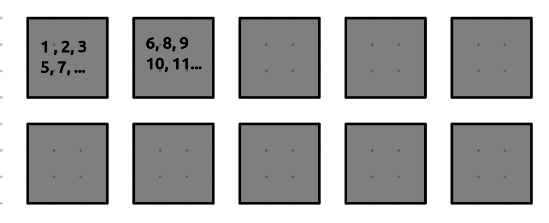
Example:

File Distribution: The master knows which files are stored on which computers. For instance:
- Computer 1 stores files 1, 2, 3, 5, 7.
- Computer 2 stores files 6, 8, 9, 10, 11 and so on ….

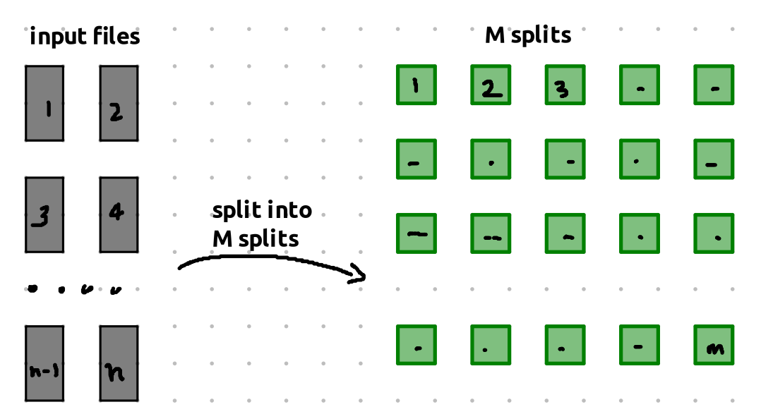
The Preprocessing Step

Before assigning tasks, the master computer pre-processes the files and splits them into map tasks. The size of each map task is typically between 16MB to 64MB.

here the pre-processing does not include reading the entire file, it mostly only processes the meta data like the size of the file.

These map tasks are chunks of the files that can be processed independently.

Task Assignment to Workers

Let’s say that the master needs to assign a task to Computer 1. If Computer 1 has File 1, the master will assign Map Task 1, which corresponds to part of File 1.

Here’s how the tasks might be split:

File 1 is split into Map Tasks 1, 2, 3, …
File 2 is split into Map Tasks 12, 13, 14, …

If Computer 1 requests a task, the master will likely assign it Map Tasks 1, 2, and 3, since File 1 is stored on Computer 1. Similarly, if Computer 2 requests a task, the master will assign it Map Tasks 12, 13, and 14, as those tasks correspond to File 2, which is stored on Computer 2.

How are Map Tasks Processed

Map Phase

The map and reduce functions are distributed to all worker computers by the master. So, every worker has a copy of these functions.

When a worker receives a map task, it reads its assigned chunk of the input file and applies the map function to it. This produces a set of key-value pairs. These key-value pairs are also known as intermediate key-value pairs.

But instead of storing all the key-value pairs in one place, the worker partitions them into R intermediate buckets — where R is the number of reduce tasks.

Each bucket contains a subset of the key-value pairs. The partitioning is usually done based on the key — often using a hash function, like:

bucket_number = hash(key) % R

This ensures that:

All values for the same key always go to the same bucket, and
Each reduce task will receive one bucket from every map worker, containing all the key-value pairs it needs to process.

Map to Reduce Transition

In this example, we have 3 reducers, so the output from each map function is split into 3 separate reduce buckets — one for each reducer.

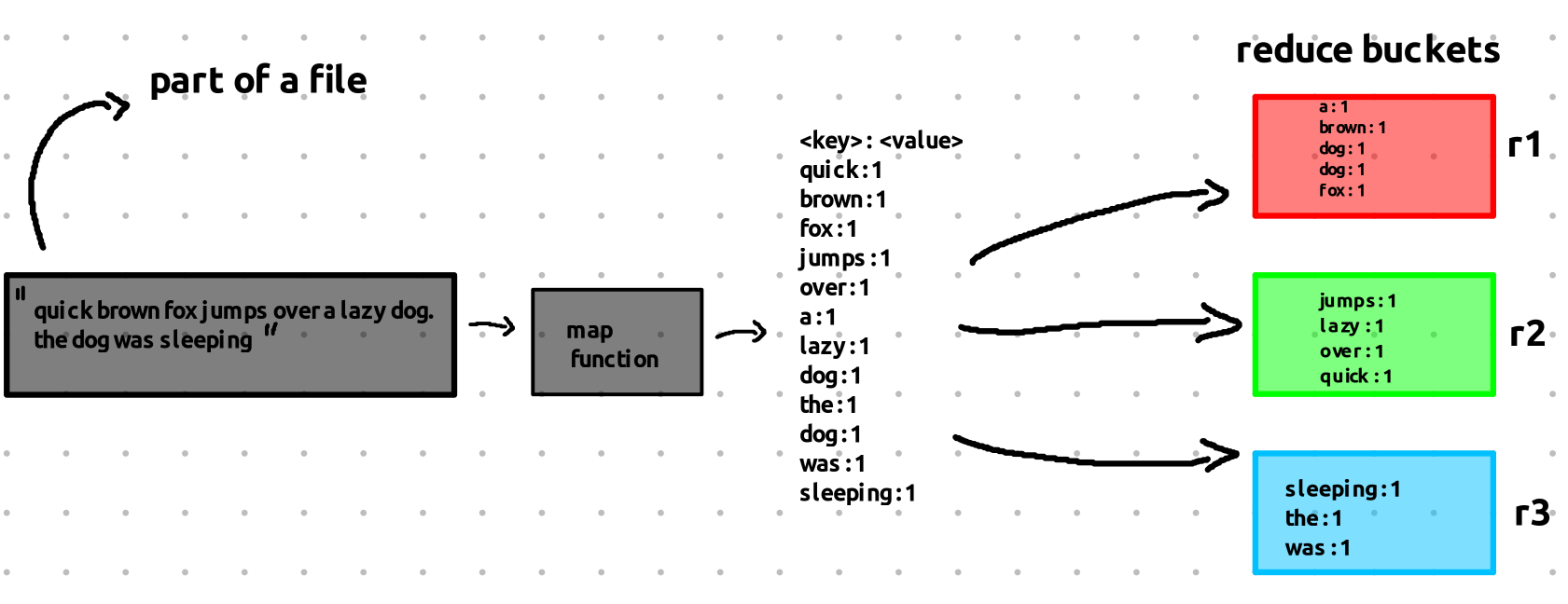
Each worker processes multiple map tasks, and each task produces key-value pairs. These key-value pairs are partitioned into three buckets, indicated by red, green, and blue in this example.

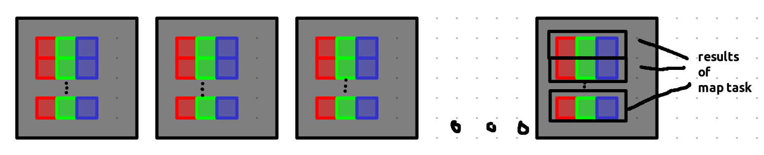
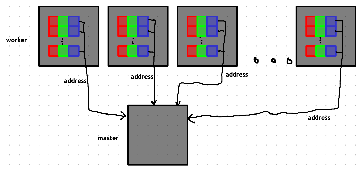
When a map task finishes, its intermediate results are stored in these buckets. The addresses (locations) of the buckets are then sent to the master — not the actual data.

Think of it like passing around pointers or references to the data — not the data itself.

Reduce Phase

Now it’s time for the reducers to step in.

The master now holds the addresses of all the intermediate results from the completed map tasks.

Don’t get confused by the visuals — each bucket shown here just represents the location of the data, not the data itself.

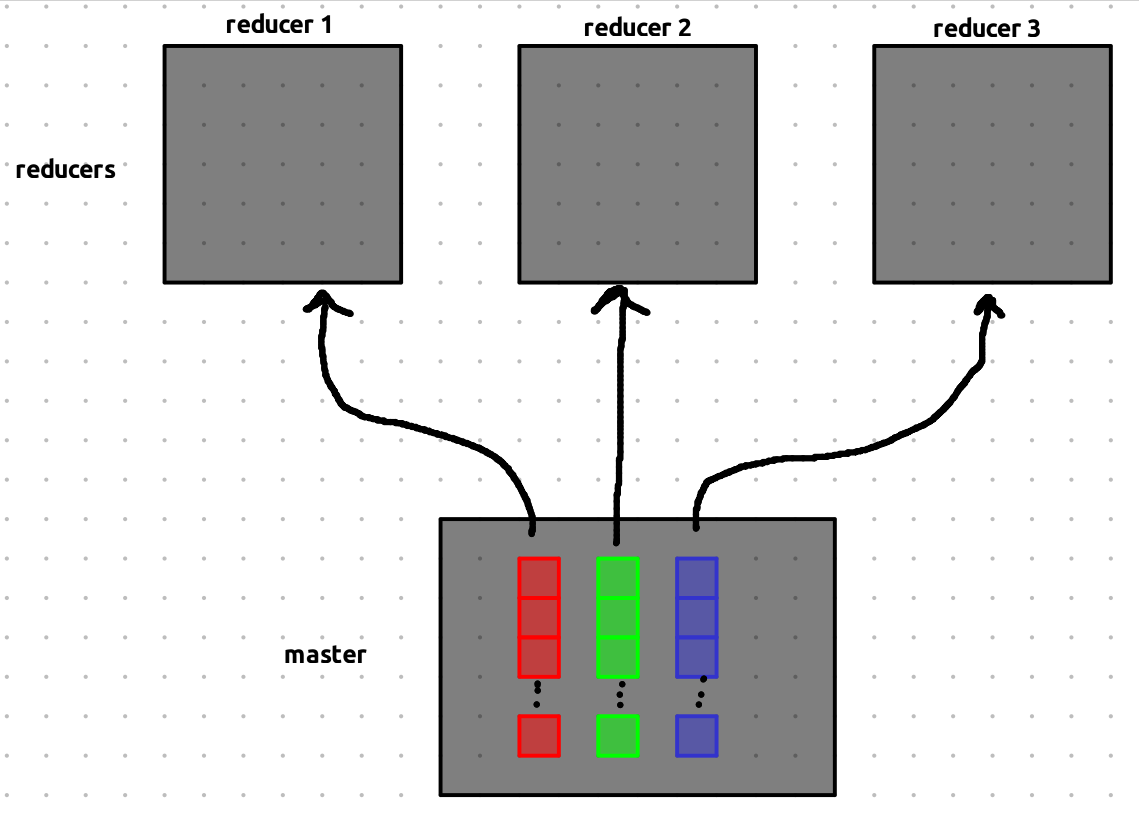
we have three reducers and master with addresses of all the results we got from computing map tasks.

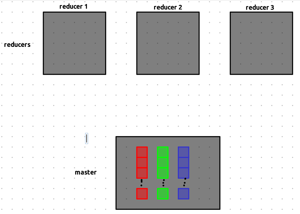
Each reducer is assigned all the buckets of a specific color (or partition):

Reducer 1 gets all red buckets,
Reducer 2 gets all green buckets,
Reducer 3 gets all blue buckets.

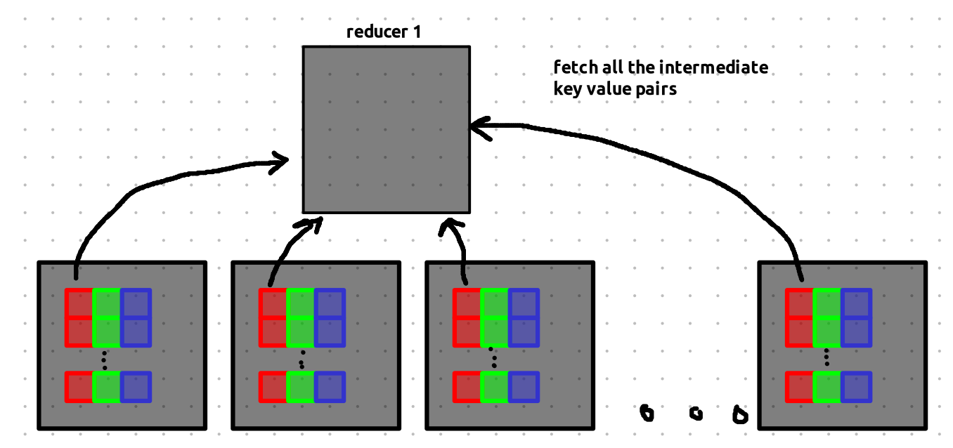
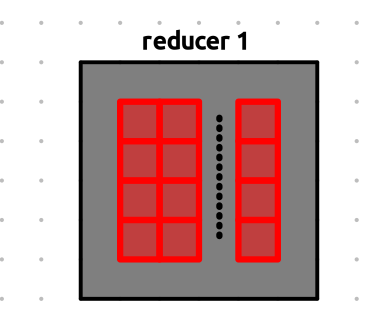
Let’s zoom into Reducer 1 to see what it does:

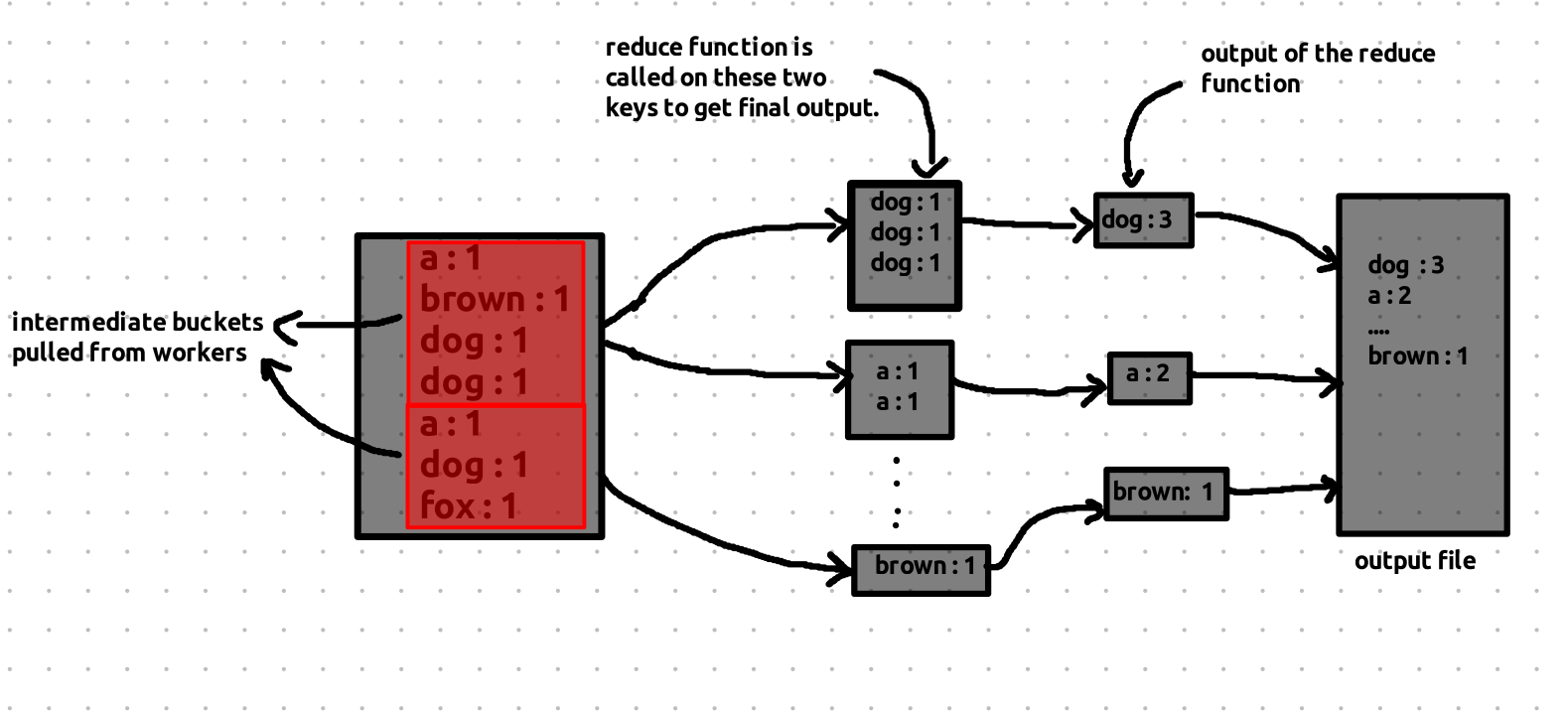
Reducer 1 now fetches all the actual data from the bucket addresses it received. Since this involves data transfer over the network, it can be a bit slow.

Once Reducer 1 collects all key-value pairs with the same key, it runs the reduce function on them and writes the final output to a file.

This same process happens in parallel for Reducers 2 and 3.

Once all reducers finish it’s DONE!

Sorting Example

now let’s see how sorting works using map reduce. the sorting confused me a bit, because i was thinking of memory constrains during the reduce phase. for the sorting to be done you must have enough space in your reducer to stored the output. in sorting the data is not moved around but the copy of the data is moved. so if the size of the data to be sorted is N we must have extra N free space left to store the result.

sorting algorithms like external merge sort and external M-way merge are used to sort and merge the data that does not fit in memory.

say you have 10 numbers range between 1-100 in 10 computer that must be sorted and you have 2 reducer. and partitioning of the intermediate keys is done using the following:

if number <= 50 {
	// bucket-1
} else {
	// bucket-2
}

here is how the state of the computers currently look like.

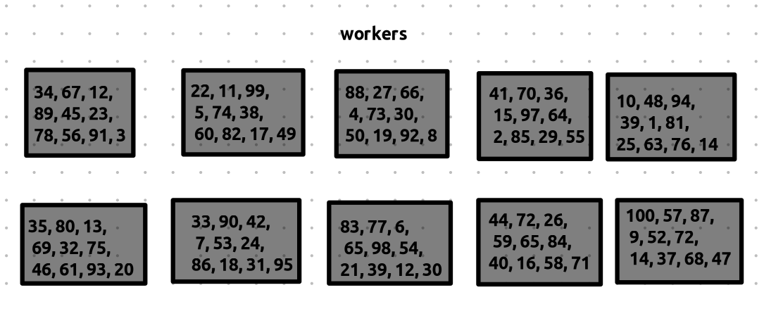
now the workers are assigned map tasks and the numbers are sorted locally, for simplicity let’s assume each worker is assigned a single map task and the map task contains includes all the numbers present in the worker.

now the numbers are sorted locally within the worker. here is current state of the workers.

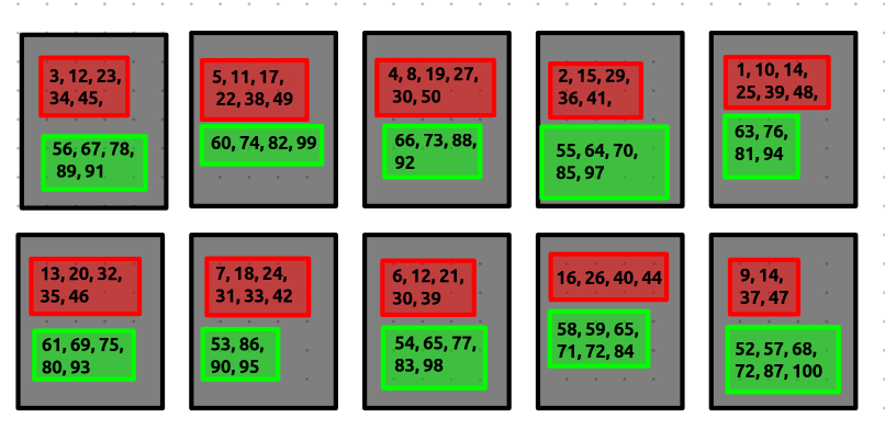
now it’s time for the reduce phase, as discussed before the workers will send back the master computer the addresses of the intermediate buckets, these addresses are sent to the reducers.

let’s zoom into the working of the reducer 1, here the reducer fetches all the buckets, and performs m-way merge, if the data is too large, it streams the data from the worker so that it’s not overloaded. and if the data is too large to fit into memory it performs m-way external merge.

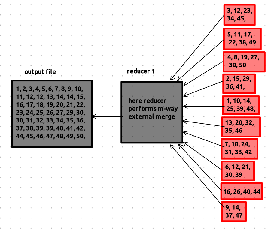
and similarly reducer 2 performs the reduce task and finally we get two output files containing numbers in the sorted order, remember these are just copy of the original number that are in the computers.

Some Interesting Stuff

Now that we’ve gone through how MapReduce works conceptually, let’s get into a practical bit — my implementation of file splitting for MapReduce. This is part of my solution for Lab 1 of the MIT 6.5840 course.

Here, I’ll talk about one interesting challenge: splitting a file into chunks that preserve full lines.

The Problem: Chunking Without Breaking Lines

Let’s say we have a file with 5 lines.

If we naively split it into fixed-size chunks, it might look like this:

As you can see, the line "they play outside." is split between two chunks. The character 'T' is in chunk 2, while the rest is in chunk 3.

This is problematic because I wanted each map task to be able to process the file line by line, which becomes difficult when lines are split across chunks.

The First (Bad) Idea 💡

At first, I thought: “Why not just read the file line by line and store those lines in tasks?”

But that turns out to be a really bad idea.

Why? Because it forces the coordinator (or master) to read the entire file — defeating the point of MapReduce, especially if you have thousands of files, each potentially gigabytes in size. This kills scalability.

The Right Approach

Instead, we should create chunks based on metadata (like file size), without reading the file content during task creation.


// creates list of MapTasks from chunks
func createMapTasks(files []string, nReduce int) []MapTask {
	slogger.Info("Creating map tasks", "nReduce", nReduce, "files", files)
	tasks := []MapTask{}
	for _, file := range files {
		chunks := createChunks(file)
		for _, chunk := range chunks {
			task := MapTask{
				Id:      uuid.NewString(),
				Chunk:   chunk,
				NReduce: nReduce,
			}
			tasks = append(tasks, task)
			slogger.Info("Created map task", "taskId", task.Id, "file", file)
		}
	}
	return tasks
}

// splits the file into chunks
func createChunks(filename string) []Chunk {
	fi, err := os.Stat(filename)
	if err != nil {
		log.Fatal("reading file stat:", err)
	}
	size := fi.Size()

	count := math.Ceil(float64(size) / float64(CHUNK_SIZE))
	tasks := []Chunk{}

	for i := range int(count) {
		task := Chunk{
			Filename: filename,
			Offset:   int64(CHUNK_SIZE * i),
			Size:     int64(CHUNK_SIZE),
		}
		tasks = append(tasks, task)
	}
	return tasks
}

Here, I’m using just the file size to define chunk boundaries — no content is read at this point.

Handling Line Boundaries When Reading

Now comes the tricky part: reading the chunk while ensuring we don’t break lines.

The logic:

If the last character of a chunk isn’t \n, it means the line continues into the next chunk.
So, the next chunk will skip the first line (since it was already partially included in the previous one).
Additionally, the current chunk might need to grab the remaining part of the line from the next chunk.

Here’s how I implemented it:

// readChunk reads a chunk and returns full lines, handling line splits at boundaries
func readChunk(task Chunk) []string {
    ...
    // Check the last byte of the previous chunk
    if task.Offset != 0 {
        prevChunkLast := make([]byte, 1)
        ...
        if prevChunkLast[0] != '\n' {
            skipStart = true
        }
    }

    ...

    // Read lines using bufio.Scanner
    scanner := bufio.NewScanner(bytes.NewBuffer(chunk))
    for scanner.Scan() {
        if i == 0 && skipStart {
            i++
            continue
        }
        lines = append(lines, scanner.Text())
    }

    // If this chunk ends in the middle of a line, grab the rest from the next chunk
    if checkNext {
        ...
    }

    return lines
}

This way, each map task processes only complete lines, and the coordinator doesn’t need to read entire files — staying true to the spirit of distributed processing.

…and then I realized — the test cases were actually applying the mapf function on the entire file directly 😅.

So technically, I didn’t even need to split the files at all. LOL.

If you’re curious, you can check out my full implementation (including this chunk-splitting logic and more) here:

👉 https://github.com/sanjayJ369/dist-db

Map-Reduce#

Naive Approach:#

MapReduce-Style Approach:#

How does MapReduce work?#

How Does MapReduce Work in Practice?#

Task Assignment and File Distribution#

Example:#

The Preprocessing Step#

Task Assignment to Workers#

How are Map Tasks Processed#

Map Phase#

Map to Reduce Transition#

Reduce Phase#

Sorting Example#

Some Interesting Stuff#

The Problem: Chunking Without Breaking Lines#

The First (Bad) Idea 💡#

The Right Approach#

Handling Line Boundaries When Reading#