Bigtable: A System That Fits It All
Paper: Bigtable: A Distributed Storage System for Structured Data (Chang et al., OSDI 2006)
Bigtable is used at Google for a wide range of projects like Google Analytics, Google Finance, Google Earth, and so on… and these different products have different forms of workload demands, from batch processing jobs to latency-sensitive jobs.
In order to do this, they provide a wide range of configurations.
First, let’s go through the architecture, and then go through the moving parts that are involved in the system and how they can be tuned.
Architecture
Here is the simplified architecture of Bigtable:
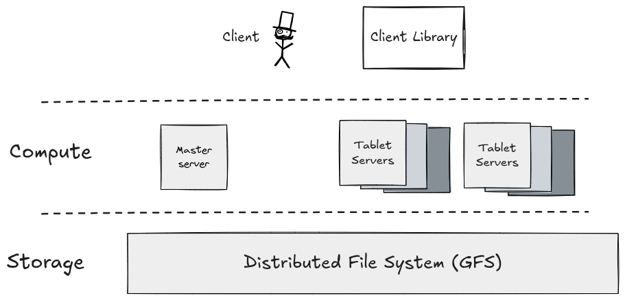
Client: We have an application which uses the Bigtable client library to interact with Bigtable.
Storage: The data is stored in a distributed file system (the Google File System); that’s our main storage.
Compute: We have a layer of servers on top of GFS which serve the data to the users, and we have a leader server which handles and manages the tablet servers. (What is a tablet? A tablet is a bunch of contiguous rows, and a tablet server is responsible for serving those rows/tablets.)
Here we follow a leader and worker pattern similar to what we have in GFS. The leader server is not a bottleneck because the interaction between the client and the leader server is kept to a minimum; all reads and writes from the clients are served by the tablet servers. The leader is only involved when doing administrative work like creating and deleting tables or column families.
The part where I got a bit confused was whether it is the tablet servers that actually store the data… but no, that’s not the case. Data is actually stored in the distributed file system, and the tablet servers are where the compute is done and where data is stored in memory until it is flushed to the file system.
Building Blocks of the System
Data Model
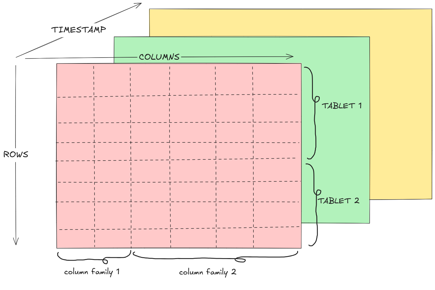
In the paper, the data model is described as a sparse, distributed, persistent, multi-dimensional sorted map (wahhhhh….)
So… it’s a map where
key => (row:string, column:string, time:int64) : value => (string)Sparse: This was a bit tricky for me to understand… the only sparse I knew was the sparse matrix, where only a few cells are filled in a large matrix. We are calling it sparse because technically we can store data in any row and any column, which is like… infinite, but we are writing and storing data only for the cells which have actual values, making it sparse.
Sorted Map: The rows are actually sorted and stored on disk.
Distributed: We are spreading compute and storage across multiple machines.
Persistent: The data is actually written to disk.
Multi-dimensional: We have time, which is the 3rd dimension.
Rows
Row keys are strings which can go up to 64KB in size. Here, the rows are stored in lexicographic order by row key. Here, a tablet is a row range which is dynamically partitioned.
Columns
Just like how we have row keys and tablets for rows, in a similar way we have column keys and column families. A set of column keys represents a column family, and data stored in all column keys of a column family is usually of the same data type. A column key is named using the following syntax: family:qualifier
Timestamp
We also store a timestamp along with the row and column key, allowing us to store different versions of the same cell. It’s a 64-bit integer that represents real time, and clients can also supply a timestamp to be used in writes.
Let’s take an example and go through the reads and writes.
We are handling an e-commerce website, and we are using Bigtable to store our data. Here, the obvious row key would be the user ID, with column families, say:
| Column Family | Example Columns | Access Pattern |
|---|---|---|
auth | auth:password_hash, auth:last_login | Accessed constantly on every request; requires low latency. |
profile | profile:name, profile:email | Accessed frequently during active sessions; requires low latency. |
history | history:order_123, history:order_124 | Large payloads; rarely accessed unless the user explicitly views past orders. |
Life of a Write
The user logs into our e-commerce website, and now we have to update their last login. The user logs in, they hit an API endpoint, and then our server uses a Bigtable client to update the last login.
Now our write request is at the Bigtable client. Where should it go? The Bigtable client needs to find the tablet server which is responsible for writing our data (this is based on the row key). But how does it know which tablet server to ask?
Here, the Bigtable client first asks the Chubby file. The Chubby file is a small file that is stored in Chubby (a distributed lock service provider), and it tells us the location of the tablet server which holds the root tablet. The root tablet stores the metadata of the other metadata tablets. This is a B+ tree, with the root node being the root tablet and the leaf nodes being the other metadata tablets. Here, the root tablet is never split, so we only ever have one root tablet.
Chubby file → root tablet → metadata tablet → target tablet serverOkay, now the client knows the root tablet. Then it gets the location of the metadata tablet from the root tablet. Then it gets the location of the tablet where the write should go (let’s call it the target tablet) from the metadata tablet.
And now, finally, our Bigtable client knows the IP of the target tablet server where the reads and writes for this row key should go.
Usually, the locations of the root tablet and the metadata tablets are cached in the client to speed things up, saving us like 3 round trips.
Now our Bigtable client has the data to write and knows where the write should go. It makes the write request to the target tablet server, and the tablet server writes the data to the memtable; before doing that, it writes the data to a write-ahead log. Once it gets an OK from the write-ahead log, it sends an OK response to the client so that we don’t keep the client waiting. And finally, our write was a success.
Here, the memtable is a sorted structure that is stored in memory. Usually, reads and writes to the memtable are of order log(n), which is pretty fast. Here, the write-ahead log is not something that’s stored on the local disk of the tablet server. Rather, the write-ahead log is something that is stored in the Google File System. The tablet server appends this write to a log file that is stored in the Google File System, so this in itself is a network call to a distributed file system.
Here, when writing to the write-ahead log, Bigtable commits a group of writes to the write-ahead log at once, and this is usually done to increase the throughput of the system.
But still, the write is in memory and in the write-ahead log. It’s not stored on disk yet. What happens is that whenever the size of the memtable goes above a certain threshold, the tablet server starts using a new memtable and freezes the old one. Then, it flushes the frozen memtable onto GFS, creating an SSTable on disk.
Obviously, we can’t keep on writing new SSTables to disk forever. What Bigtable does is periodically combine several SSTables and merge them into a new SSTable, reclaiming space in the process by doing garbage collection.
Life of a Read
Reads are very similar to writes. We just get the location of the target tablet server in a similar way. If we want to read something, we first need to know the row key. Based on the row key, we follow the Chubby file → root tablet → metadata tablet flow to get the location of our target tablet server. The Bigtable client asks the target tablet server for what we want.
Then, the tablet server looks at the memtable and the subsequent SSTables to find the row and returns it.
Tuning and Performance (Knobs)
Locality Groups
This allows the user to group multiple column families together into one locality group. Each locality group has its own SSTable; the reason for this is mainly that we don’t want the access patterns of one column to affect another.
If we take a quick look at our example, we have auth, which is something that will be frequently used by the customer, and we also have history, which is something that is rarely used by the user.
If both of these were in the same SSTable, whenever we access the auth data, we would be forced to go through the history values as well, as they are in the same SSTable.
Here, what we can do is use different locality groups, one for history and one for auth, and Bigtable also allows us to have different configs for each locality group.
One configuration is that we can keep the SSTables in memory, so the auth SSTables will stay in memory; this is suitable for small pieces of data that are accessed frequently.
Compression
Bigtable allows compression to be set per locality group, so that we can turn on compression for history and keep compression off for auth, based on their access patterns. Auth is something that is used more frequently, and you might not want to introduce something like an encoding and decoding process during writes and reads, which would slow it down.
Here, we can turn on compression for order history, as most of the orders store similar data, like the names of the products, the addresses, and so on. Here, it will be really useful because of the two-pass compression which Bigtable allows. They found a nearly 10:1 reduction in space, with reasonable encoding and decoding times.
Bloom Filters
Bloom filters are a probabilistic data structure that’s widely used in databases. Here, the data for a row can be spread across the memtable and several SSTables. The memtable is in memory, so checking it is cheap, but checking each SSTable means a disk read, and going through every one of them to find a value for a given row/column pair would be really expensive.
Instead, if we use a Bloom filter, it tells us whether the row/column pair might be present in an SSTable, or whether it’s definitely not present in that SSTable. Bloom filters save us a lot of disk reads, but they cost us some memory.
Bigtable lets us turn Bloom filters on or off for each locality group.
Summary
Going back to where we started: how does one system handle such a wide variety of workloads? Bigtable gives us knobs that we can tune to fit our workloads.
We have locality groups, where we can group similar column families together. We can use different compression for different locality groups. And we can turn Bloom filters on or off for each of them. In our e-commerce example, auth stays in memory with no compression, and history gets compressed and stays on disk… same table, but tuned in two completely different ways.
To get all this, Bigtable makes a lot of tradeoffs. One important one is that transactions are limited to a single row. A write to one row is atomic, but if we want to update two rows together, Bigtable won’t help us there.
We also don’t have secondary indexes. We only have one index, and that’s the row key. So we can either look up a row key or scan a range of row keys, and that’s it. This makes choosing the row key really important. Since rows are sorted, if we use something like a timestamp as the row key, all the new writes go to the same tablet server, and that server becomes a hotspot.
Even with these tradeoffs, a lot of systems today are built on ideas from Bigtable. HBase is basically an open-source Bigtable, and the memtable → SSTable → compaction flow is what LevelDB, RocksDB and TidesDB use too.